Scicos > Book: Modeling and Simulation in Scilab/Scicos
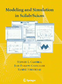
 Modeling and Simulation in Scilab/Scicos
by Stephen L. Campbell, Jean-Philippe Chancelier, and Ramine Nikoukhah
Purchase at: Springer or Amazon . ISBN 0-387-27802-8
Download the examples
Book cover [PDF]
Table of contents [PDF]
Chapter 7: Scicos, Getting started [PDF]
The objective of this book is to provide a tutorial for the use of Scilab/Scicos with a special emphasis on modeling and simulation tools. While it will provide useful information to experienced users it is designed to be accessible to beginning users from a variety of disciplines. Students and academic and industrial scientists and engineers should find it useful.
The book is divided into two parts. The first part concerns Scilab and includes a tutorial covering the language features, the data structures and specialized functions for doing graphics, importing, exporting data and interfacing external routines. It also covers in detail Scilab numerical solvers for ordinary differential equations and differential-algebraic equations. Even though the emphasis is placed on modeling and simulation applications, this part provides a global view of Scilab. The second part is dedicated to modeling and simulation of dynamical systems in Scicos. This type of modeling tool is widely used in industry because it provides a means for constructing modular and reusable models. This part contains a detailed description of the editor and its usage, which is illustrated through numerous examples. All codes used in the book are made available to the reader.
|
|
||
| Part I | Scilab | |
|
|
||
| 1 | General Information | 3 |
| 1.1 | What Is Scilab? | 3 |
| 1.2 | How to Start? | 4 |
| 1.2.1 | Installation | 4 |
| 1.2.2 | First Steps | 4 |
| 1.2.3 | Line Editor | 5 |
| 1.2.4 | Documentation | 6 |
| 1.3 | Typical Usage | 6 |
| 1.4 | Scilab on the Web | 7 |
| 2 | Introduction to Scilab | 9 |
| 2.1 | Scilab Objects | 11 |
| 2.1.1 | Matrix Construction and Manipulation | 12 |
| 2.1.2 | Strings | 17 |
| 2.1.3 | Boolean Matrices | 19 |
| 2.1.4 | Polynomial Matrices | 20 |
| 2.1.5 | Sparse Matrices | 21 |
| 2.1.6 | Lists | 22 |
| 2.1.7 | Functions | 26 |
| 2.2 | Scilab Programming | 27 |
| 2.2.1 | Branching | 28 |
| 2.2.2 | Iterations | 29 |
| 2.2.3 | Scilab Functions | 31 |
| 2.2.4 | Debugging Programs | 35 |
| 2.3 | Input and Output Functions | 37 |
| 2.3.1 | Display of Variables | 37 |
| 2.3.2 | Formatted Input and Output | 38 |
| 2.3.3 | Input Output in Binary Mode | 40 |
| 2.3.4 | Accessing the Host System | 42 |
| 2.3.5 | Graphical User Interface | 43 |
| 2.4 | Scilab Graphics | 48 |
| 2.4.1 | Basic Graphing | 48 |
| 2.4.2 | Graphic Tour | 49 |
| 2.4.3 | Graphics Objects | 53 |
| 2.4.4 | Scilab Graphics and \LaTeX | 56 |
| 2.4.5 | Old Graphics Style | 60 |
| 2.5 | Interfacing | 62 |
| 2.5.1 | Linking Code | 63 |
| 2.5.2 | Writing an Interface | 66 |
| 2.5.3 | Dynamic Loading | 69 |
| 3 | Modeling and Simulation in Scilab | 73 |
| 3.1 | Types of Models | 73 |
| 3.1.1 | Ordinary Differential Equations | 73 |
| 3.1.2 | Boundary Value Problems | 74 |
| 3.1.3 | Difference Equations | 75 |
| 3.1.4 | Differential Algebraic Equations | 76 |
| 3.1.5 | Hybrid Systems | 77 |
| 3.2 | Simulation Tools | 78 |
| 3.2.1 | Ordinary Differential Equations | 78 |
| 3.2.2 | Boundary Value Problems | 90 |
| 3.2.3 | Difference Equations | 95 |
| 3.2.4 | Differential Algebraic Equations | 98 |
| 3.2.5 | Hybrid Systems | 100 |
| 4 | Optimization | 107 |
| 4.1 | Comments on Optimization and Solving Nonlinear Equations | 107 |
| 107 | ||
| 108 | ||
| 4.2 | General Optimization | 108 |
| 4.3 | Solving Nonlinear Equations | 112 |
| 4.4 | Nonlinear Least Squares | 113 |
| 113 | ||
| 114 | ||
| 4.5 | Parameter Fitting | 117 |
| 4.6 | Linear and Quadratic Programming | 119 |
| 4.6.1 | Linear Programs | 119 |
| 4.6.2 | Quadratic Programs | 120 |
| 4.6.3 | Semidefinite Programs | 120 |
| 4.7 | Differentiation Utilities | 120 |
| 4.7.1 | Higher Derivatives | 122 |
| 5 | Examples | 125 |
| 5.1 | Modeling and Simulation of an N-Link Pendulum | 125 |
| 5.1.1 | Equations of Motion of the N-Link Pendulum | 126 |
| 5.1.2 | Generated Code and Simulation | 130 |
| 5.1.3 | Maple Code | 133 |
| 5.2 | Modeling and Simulation of a Car | 135 |
| 5.2.1 | Basic Model | 135 |
| 5.2.2 | Equations of Motion | 136 |
| 5.2.3 | Simulation Model | 138 |
| 138 | ||
| 5.2.4 | Scilab Implementation | 139 |
| 5.2.5 | Simulation Result | 141 |
| 5.3 | Open-Loop Control to Swing Up a Pendulum | 142 |
| 5.3.1 | Model | 142 |
| 5.3.2 | Control Problem Formulation | 142 |
| 5.3.3 | Optimization Problem | 143 |
| 5.3.4 | Implementation in Scilab | 145 |
| 5.4 | Parameter Fitting and Implicit Models | 147 |
| 5.4.1 | Mathematical Model | 148 |
| 5.4.2 | Scilab Implementation | 148 |
|
|
||
| Part II | Scicos | 157 |
|
|
||
| 6 | Introduction | 159 |
| 7 | Getting Started | 163 |
| 7.1 | Construction of a Simple Diagram | 163 |
| 7.1.1 | Running Scicos | 163 |
| 7.1.2 | Editing a Model | 163 |
| 7.1.3 | Diagram Simulation | 165 |
| 7.1.4 | Changing Block Parameters | 166 |
| 167 | ||
| 168 | ||
| 7.2 | Symbolic Parameters and Context | 169 |
| 173 | ||
| 7.3 | Hierarchy | 173 |
| 7.3.1 | Placing a Super Block in a Diagram | 173 |
| 7.3.2 | Editing a Super Block | 174 |
| 7.4 | Save and Load | 175 |
| 7.4.1 | Scicos File Formats | 175 |
| 7.4.2 | Super Block and Palette | 176 |
| 7.5 | Synchronism and Special Blocks | 176 |
| 8 | Scicos Formalism | 179 |
| 8.1 | Activation Signal | 179 |
| 8.1.1 | Block Activation | 179 |
| 8.1.2 | Activation Generation | 181 |
| 8.2 | Inheritance | 182 |
| 8.3 | Always Active Blocks | 183 |
| 8.4 | Constant Blocks | 184 |
| 8.5 | Conditional Blocks | 184 |
| 9 | Scicos Blocks | 189 |
| 9.1 | Block Behavior | 189 |
| 9.1.1 | External Activation | 189 |
| 190 | ||
| 191 | ||
| 191 | ||
| 9.1.2 | Always Activation | 191 |
| 9.1.3 | Internal Zero-Crossing | 192 |
| 9.2 | Blocks Inside Palettes | 192 |
| 9.3 | Modifying Block Parameters | 193 |
| 9.4 | Super Block and Scifunc | 193 |
| 9.4.1 | Super Blocks | 193 |
| 9.4.2 | Scifunc | 194 |
| 9.5 | Constructing New Basic Blocks | 194 |
| 9.5.1 | Interfacing Function | 195 |
| 195 | ||
| 196 | ||
| 196 | ||
| 9.5.2 | Computational Function | 197 |
| 201 | ||
| 206 | ||
| 9.5.3 | Saving New Blocks | 207 |
| 9.6 | Constructing and Loading a New Palette | 207 |
| 10 | Examples | 209 |
| 10.1 | Predator Prey Model | 209 |
| 10.2 | Control Application | 210 |
| 10.3 | Signal Processing Application | 213 |
| 10.4 | Queuing Systems | 216 |
| 10.5 | Neuroscience Application | 218 |
| 10.6 | A Fluid Model of TCP-Like Behavior | 220 |
| 10.7 | Interactive GUI | 221 |
| 11 | Batch Processing in Scilab | 227 |
| 11.1 | Piloting Scicos via Scilab Commands | 227 |
| 11.1.1 | Function scicosim | 228 |
| 11.1.2 | Function scicos_simulate | 232 |
| 11.2 | Data Sharing | 233 |
| 11.2.1 | Context Variables | 234 |
| 11.2.2 | Input/Output Files | 234 |
| 11.2.3 | Global Variables | 236 |
| 11.3 | Examples | 237 |
| 11.4 | Steady-State Solution and Linearization | 243 |
| 11.4.1 | Scilab Function steadycos | 247 |
| 11.4.2 | Scilab Function lincos | 248 |
| 12 | Code Generation | 253 |
| 12.1 | Code Generation Procedure | 253 |
| 12.2 | Limitations | 257 |
| 12.2.1 | Continuous-Time Activation | 257 |
| 12.2.2 | Synchronicism | 258 |
| 12.3 | A Look Inside | 258 |
| 258 | ||
| 259 | ||
| 260 | ||
| 260 | ||
| 260 | ||
| 12.4 | Some Pitfalls | 260 |
| 12.5 | Applications | 263 |
| 13 | Debugging | 267 |
| 13.1 | Error Messages | 267 |
| 13.1.1 | Block Errors | 267 |
| 13.1.2 | Errors During Numerical Integration | 268 |
| 13.1.3 | Other Errors | 269 |
| 269 | ||
| 269 | ||
| 13.2 | Debugging Tools | 269 |
| 13.3 | Examples | 270 |
| 13.3.1 | Log File | 271 |
| 13.3.2 | Animation | 271 |
| 14 | Implicit Scicos and Modelica | 273 |
| 14.1 | Introduction | 273 |
| 14.2 | Internally Implicit Blocks | 275 |
| 14.3 | Implicit Blocks | 275 |
| 14.3.1 | Scicos Editor | 276 |
| 14.3.2 | Scicos Compiler | 276 |
| 14.3.3 | Block Construction | 276 |
| 14.4 | Example | 277 |
| A | Inside Scicos | 281 |
| A.1 | Scicos Editor | 281 |
| A.1.1 | Main Editor Function | 281 |
| Example | 282 | |
| A.1.2 | Structure of scs_m | 283 |
| 285 | ||
| 286 | ||
| A.2 | Scicos Complier | 286 |
| A.2.1 | First Compilation Stage | 286 |
| A.2.2 | Second Compilation Stage | 287 |
| A.2.3 | Structure of %cpr | 287 |
| A.2.4 | Partial Compilation | 290 |
| A.3 | Scicos Simulator | 291 |
| B | Scicos Blocks of Type 5 | 293 |
| B.1 | Type 5 Block for the Bouncing Ball Example | 293 |
| B.2 | Animation Block for the Cart Pendulum Example | 294 |
| C | Animation Program for the Car Example | 299 |
| D | Extraction Program for the LaTeX Graphic Example | 301 |
| E | Maple Code Used for Modeling the N-Link Pendulum | 303 |
| References | 307 | |
| Index | 309 | |

 Download