Scicos Codegeneration
fr - eng

CodeGeneration - Scicos Code Generation

Module

• Scicos

Contents

• CodeGeneration - Scicos Code Generation
  • Module
  • Background
  • Scicos Overview
  • Functional approach
  • Code generation implementation
  • Inside the editor
  • Use and definition of external libraries and additional compiler flag(s)
  • List of the main generated files
  • Code generation from the ScicosLab prompt
  • Use of the ScicosLab interfacing function for the standalone
  • Use the loader script to reload the generated codes inside Scicos/ScicosLab
  • Standalone executable
  • Authors

Background

Scicos is a modeler/simulator of hybrid dynamical systems. It can simulate a wide variety of systems, including in a same process of simulation, discrete and continuous time dynamics.

Scicos can solve non-linear differential equations described by Ordinary Differential Equations (ODE), Differential Algebraic Equations (DAE) and Discrete Difference Equations. With Scicos one can model hybrid dynamical systems by using block diagram schematics and/or by using the modelling language Modelica. In both cases the user can generate C code from the model description.

An hybrid dynamical system can be described by separating the continuous time from the discrete time dynamics. For a system using ODEs, we can write the continuous time part as :

$$\begin{eqnarray} y\left(t\right) & = & f\left(t,x\left(t\right),z\left(t_{k}\ri... ...t(t,x\left(t\right),z\left(t_{k}\right),u\left(t\right),p\right) \end{eqnarray}$$

where t is the continuous time, y(t) is a vector of outputs, u(t) is a vector of inputs, x(t) is a vector of states, dot(x)(t) is the vector of the derivative states, z(tk) is a vector of discrete states and p a vector of constant parameters. f and h are functions that define non-linear relation between variables. For a system using DAEs, we can write the continuous time part as :

$$\begin{eqnarray} 0 & = & f\left(t,y\left(t\right),x\left(t\right),z\left(t_{k}\... ...t(t,x\left(t\right),z\left(t_{k}\right),u\left(t\right),p\right) \end{eqnarray}$$

where (3) defines algebraic relations.

For the discrete time part, one can write :

$$\begin{eqnarray} y\left(t_{k}\right) & = & f\left(t_{k},x\left(t_{k}\right),z\l... ...ft(t_{k}\right),z\left(t_{k}\right),u\left(t_{k}\right),p\right) \end{eqnarray}$$

where tk is the discrete time, gc and gd are respectively functions for the states vector and the discrete states vector. Note that here have written x(t+) instead of x(tk+1) for (6) because we assume that a discrete jump occurs during the continuous time integration of the state vector.

In a Scicos simulation, the delay between two discrete instants tk+1 and tk is not necessary constant. Such instants are called output events date and are computed by primary sources of activation. These sources are defined by :

$$\begin{eqnarray} t_{k+1} & = & k\left(t_{k},x\left(t_{k}\right),z\left(t_{k}\right),u\left(t_{k}\right),p\right) \end{eqnarray}$$

and can also be defined with a continuous time equation by using zeros crossing threshold related to continuous time states or inputs :

$$\begin{eqnarray} t_{k+1} & = & \text{inf} \{ t > t_k \text{ such that } 0 = g_{... ...,x\left(t\right),z\left(t_{k}\right),u\left(t\right),p\right) \} \end{eqnarray}$$

Scicos Overview

In Scicos, hybrid dynamical systems defined by the previous equations, can be modeled by a block diagram graphic editor :

Figure 1: A Scicos block diagram

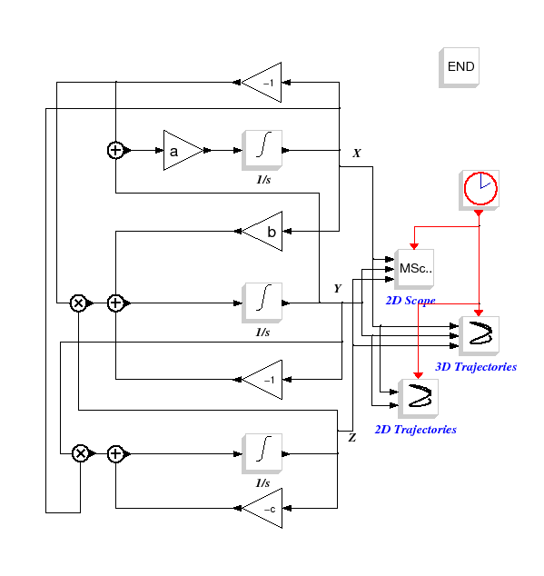
This diagram models the Lorentz's system defined by the following set of equations :

$$\begin{eqnarray} \dot{x}(t) & = & a\left(-x(t)+y(t)\right)\\ \dot{y}(t) & = & bx(t)-y(t)-x(t)y(t)\\ \dot{z}(t) & = &-cx(t)+x(t)y(t) \end{eqnarray}$$

To simulate the dynamical system, the diagram (or its Modelica description if this high level language is used) must be compiled to translate the symbolic description in a compiled structure (or tree) that can be used both by a simulator and a code generator.

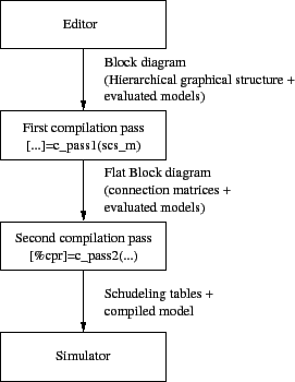
In the current Scicos version, the following flowchart shows a top-down view of the main parts of the modeler/simulator :

Figure 2: Flowchart Scicos implementation

• The output of the editor is a structure that corresponds to the hierarchical main diagram. It contains informations related to graphical objects (e.g. blocks, links, ...) appearing in the figure. Additional informations are set in that structure such that simulation parameters, code generation properties, etc...

• A first step of the compiling process realizes a flat diagram structure. In the hierarchical representation of the Scicos editor some blocks (called super block) are allowed to contain other diagram structure. During that step, all graphical informations not needed for simulation are removed from the output structure.

• Then a second pass in the compiler realizes the scheduling of blocks in the flat diagram. The output compiled structure have all informations needed for the simulation.

Functional approach

A more detailed flowchart of the Scicos hybrid dynamical systems toolbox is shown in figure 3.

Figure 3: Flowchart : Functional approach

• In the left part is shown how the Scicos code generation interacts with the compiler and the simulator. With the informations provided by the compiler, two codes are generated :
  • one is a computational function. This code can directly be called by the simulator. That code calls the Standard/user's blocks computational functions and/or the computational function provided by the Scicos/Modelica implementation.
  • the second code is called standalone code. It is a code which includes both the calls to the Standard/user's blocks computational functions (and/or the computational function provided by the Scicos/Modelica implementation) and simulator parts needed to achieve the simulation.

Code generation implementation

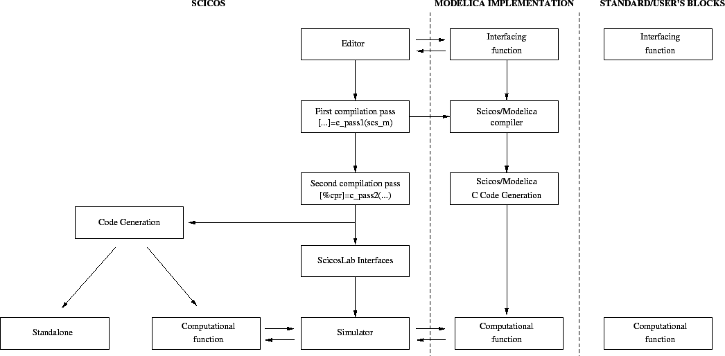
Figure 4 displays the current Scicos code generation implementation.

Figure 4: Flowchart : code generation implementation

Inside the editor

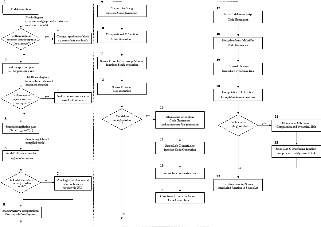
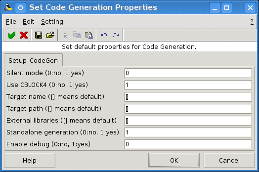
In the editor, the C code generation can be achievied through a super-block or an complete top-level diagram. The various steps of code generation are not visible by the user. Finally, the generated codes are automatically compiled and dynamically linked inside Scicos and ScicosLab.

Default properties definition

Description

Before running the code generation process, the user can set some parameters that will overload the default properties of the generation. That parameters can be set with a GUI which appears in the Scicos menu 'Diagram', option 'Set Code Gen Properties' or with the context menu (also called Popup Menu) when user right click on a super-block and use the menu 'Super Block Properties'.

Dialog box

Figure 5: The diagram GUI of the code generation

• Silent mode (0:no, 1:yes) : If set to 1, this parameter means that no GUI will be displayed during the code generation processes. This is useful when running code generation in batch mode.

• Use CBLOCK4 (0:no, 1:yes) : This parameter enables the use of a generic type 4 C block for the generation of the Scicos interfacing function associated with the newly created block.

• Target name ([] means default) : By default, a name is given for the generated code according to the title of the diagram or the title of the super-block. This dialog parameter overload the default name chosen by the code generation.

• Target path ([] means default) : By default, a name is chosen for the target path of the generated code, according to the title of the diagram or the title of the super-block. This dialog parameter overload the default path chosen by the code generator. This is useful for example to set it at 'TMPDIR' when doing a long sequence of tests.

• External libraries ([] means default) : With that parameter, the user can affect external libraries for a diagram or for a super-block. This parameter doesn't remove the external libraries set by the global Scicos variable %scicos_libs.

• Standalone generation (0:no, 1:yes) : One can disable the standalone code generation with that parameters.

• Enable debug (0:no, 1:yes) : That parameters is for use only by experts. If set to 1, additionnal code is generated in the computational function and in the standalone code for the debugging purpose.

Use of the main GUI

Description

In the Scicos editor, the code generation begins by choosing the 'Code Generation' item in the Scicos menu 'Tools' and then by clicking in a void area (for an entire diagram generation) or by cliking on a super-block. The user can also first select the super-block that must be generated and then use the popup Menu (mouse right click) and choose the option 'Code Generation'.

Then a dialog box appears, asking the user to set some parameters concerning the code generation. Most of that parameters are default values or values set in the diagram GUI.

Dialog box

Figure 6: The main GUI of the code generation

• New block's name : That parameter is a string which defines the new name of the Scicos block that will be generated inside the ScicosLab environment. It will serve as a main identifier concerning names given for the generated functions and files.
  For example, if we choose to name our block 'Rdnom' :
  • The Scicos interfacing function will be called 'Rdnom_c' and its associated file 'Rdnom_c.sci',
  • the type 4 computational function will be called 'Rdnom' and its associated file 'Rdnom.c',
  • the simulation function of the standalone code will have the name 'Rdnom_sim' and its file 'Rdnom_standalone.c',
  • the ScicosLab interfacing function of the Standalone will be called 'Rdnom' and its associated file 'intRdnom_sci.c',
  • the Makefiles will have the names 'Makefile_Rdnom(.lcc/.mak)' and 'Makefile_intRdnom(.lcc/.mak)' to respectively compile the computational function/standalone code and the ScicosLab interfacing function,
  • the loader script that reload generated functions in the ScicosLab environment will be called 'Rdnom_loader.sce',
  • and etc...

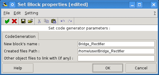
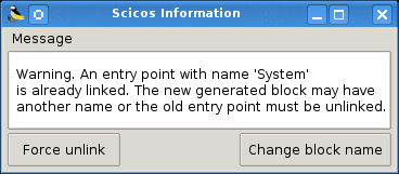
  Note that some restrictions still exist concerning the name of the block :

  • The name cannot contains space, the ``.'' character and the ``-'' character. If such characters are used, then the main GUI will substitute them by the underscore character (``_'') and a message will be displayed to ask to the user to change the new name if needed.
  • If a computational function with a the same name have already been dynamically linked in the ScicosLab environment, then the GUI displays the following message for the user :
    
    Figure 7: GUI asking to the user to change the name of the generated codes
    • Change block name : For the first choice, the GUI will automatically rename the block'name by adding a 'x' character to the end of the characters string, with 'x' an increasing number corresponding to the number of time taht the block have been generated or dynamically linked into ScicosLab. The user will have the choice to rename it if needed.

    • Force unlink : that button allows to unlink the previous computational function from ScicosLab. The new will then replace it.

• Created files path : that parameter gives the target path. In that path, the files will be generated and compiled. If that path doesn't exist, the code generator will created it. If it can't, a message will be displayed to the user and the generation will stop.

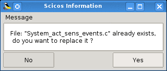
  Note that some restrictions still exist concerning the name of the path :

  • The name can't contains space character. If a space is used, then the main GUI will substitute it by the underscore character (``_'') and a message will be displayed to ask to the user to change the new path if needed.

• Other files to link with (if any) : that parameter is a character string row vector. It is used to spectify the paths and names of additionnal external libraries. That libraries enclose compiled user's computational functions and other functions needed to compile and link the standalone generated code. For each library, a static and a shared version are needed. The shared library is for the dynamical link into ScicosLab, and the static is to compile the standalone executable.

  The libraries must have file extensions ".dll" for the windows operating systems (OS), and ".so" for the Linux OS. The generator will then automatically look at for static libraries with file extensions ".lib" for Windows OSs and ".a" for Linux OS.

  If that lastest files are not found, the GUI send a message to the user and the generation is aborted.

• Additional compiler flag(s) : this parameter defines an additional option for the C compiler. This can be useful for specifying a directory to include (needed for header file) and/or to include libraries (like '-lstdc++' under Linux OS).

When the user has informed all the GUI parameters, he accepts by click in the 'Ok' button, or by pressing the key 'Enter'.
But sometimes, the generation or the compilation processes will fail. In such cases error or warning messages are send to the user. The most encountered warning in the Scicos code generation is when the user generates code over an already generated block (with same name and same target path). In that case, the following dialog box appears and ask to the user if the file for the actuators/sensors routines 'Rdnom_act_sens_events.c' must be erased.

Figure 8: GUI asking to the user to rewritte the Actuator/sensor routines

Use and definition of external libraries and additional compiler flag(s)

The use of the field entries 'Other files to link with (if any)' and 'Additional compiler flag(s)' in the main GUI of the code generation can be sometimes difficult and boring when the diagram is composed of lot of user's blocks that need many external libraries.

In Scicos, the global variable %scicos_libs can be used to inform external libraries from the ScicosLab prompt just before launching the Scicos editor. The global variable %scicos_cflags is used as a compiler flag.

Typically it can be used in a 'loader.sce' script file that is in charge of loading user's function like interfacing functions and computational functions.

An example of use of such a script is given below :

099  ...
0100 if MSDOS then
0101   libnam = ['mylib1.dll','mylib2.dll']
0102 else
0103   libnam = ['mylib1.so','mylib2.so']
0104 end
0105
0106 if %scicos_libs<>[] then
0107   for i=1:size(libnam,2)
0108     if find(libnam(i)==%scicos_libs)==[] then
0109       %scicos_libs=[%scicos_libs,libnam(i)]
0110     end
0111   end
0112 else
0113   %scicos_libs=libnam
0114 end
0115
0116 if ~MSDOS then %scicos_cflags=[%scicos_cflags,'-lstdc++']; end
0117...

When this variables are informed, the code generator of Scicos will automatically use it during the link and compile processes. The dialog parameter 'Other files to link with (if any)' of the main GUI will be then set with the contents of %scicos_libs and the dialog parameter 'Additional compiler flag(s)' with the content of the variable %scicos_cflags.

Finally, one can say that when the user generates a new block with the code generation, then the output library of the new block will be automatically added at the end of the %scicos_libs content. That behaviour is for users that use the generated block inside other blocks or diagram to be generated.

List of the main generated files

Files	Description
Rdnom.c	Scicos computational function
Rdnom_c.sci	Scicos interfacing function
Rdnom_standalone.c	Standalone code
Rdnom_act_sens_events.c	Actuators/sensors routines (shell/files)
Rdnom_void_io.c	Actuators/sensors routines (generic C structure)
Rdnom_params.dat	Parameters standalone file (``little endian binary'')
IntRdnom_sci.c	ScicosLab/standalone interfacing function
Makefile_Rdnom (lcc.mak/mak)	Makefile for the computational function and the standalone codes
Makefile_intRdnom (lcc.mak/mak)	Makefile for the ScicosLab/standalone interfacing function
Rdnom_loader.sce	ScicosLab script to reload the generated code inside ScicosLab

Code generation from the ScicosLab prompt

Description

The code generation of an entire diagram can be done without running the Scicos editor. This feature can be automatically realized with the ScicosLab macro scicos_codegeneration from the Scicoslab prompt. Before use this function the desired diagram must be loaded into ScicosLab, for example by using the 'load' command for a diagram included in a '.cos' file. After the generation, the resulting diagram can be loaded in scicos with ->scicos(scs_m);. Default parameters for code generation can be set with the help of the 'Params' argument.

Calling Sequence

[ok,scs_m,%cpr] = scicos_codegeneration(scs_m,Params)

Parameters

• scs_m : Scicos diagram (obtained, e.g., by 'load file.cos').
• Params : A list of properties for scicos code generation.
  • Params(1) : silent_mode : if 1 then no message are displayed during the code generation and default values are taken for the target directory and names.
  • Params(2) : cblock : if set to 1, the generated block is replaced by a CBLOCK4 that enclosed the generic parameters and the generated computational function.
  • Params(3) : rdnom : sets the default name for the generated code.
  • Params(4) : rpat : sets the default target path for the generated code.
  • Params(5) : libs : sets the additional external libraries needed by code generation.
  • Params(6) : opt : if 0, then the standalone code will not be generated -default 1-.
  • Params(7) : enable_debug : says if additionnal code must be generated to debug generated codes.
• ok : Flag to say if the code generation is successfull.
• scs_m : The resulting diagram, that contains the generated block if any.
• %cpr : The resulting compiled structure.

Use of the ScicosLab interfacing function for the standalone

The code generation of Scicos generates both a computational function and a standalone code. In the generation process, when the user choose to generate the standalone code, it is automatically compiled and dynamically linked in the ScicosLab environment. Then the standalone code can be used by the way of a ScicosLab interfacing function which is also generated, compiled and dynamically linked in the same time than the standalone code. The ScicosLab interfacing function is a C function and is automatically added to the list of the ScicosLab functions with the help of the function addinter.

For a generated code called 'Rdnom', such a function will have the following calling sequence in ScicosLab for an entire diagram generation :

[out1,out2,...,outX]=Rdnom(in1,in2...,inX,[,tf][,fil])

with

• out1,out2,...,outX : the output signals corresponding to the X actuators.
• in1,in2...,inX : the input vector or matrix corresponding to the X sensors.
• tf : the final time of the simulation (optional).
• file : the path and name of the binary data file that contains the parameters and initial states values (optional).

and the following calling sequence for a super-block code generation :

[out1,out2,...,outX]=Rdnom(in1,in2...,inX,[,te][,tf][,h][,solver])

with

• out1,out2,...,outX : the output signals corresponding to the X actuators.
• in1,in2...,inX : the input vector or matrix corresponding to the X sensors.
• te : the sampling time (optional, default 0.1).
• tf : the final time of the simulation (optional, default 30).
• h : solver step (optional, default 0.001).
• solver : solver type, 1:Euler, 2:Heun, 3:R.Kutta (optional, default 3).

The output signals are scilab structures composed by two fields : time and values. After have running the interfacing function, on can compute, e.g., an output signal :

-->out1=Discrete_KalmanFilter()
out1  =

values: [15000x3 constant]
time: [15000x1 constant]

The field values contains the data stored during the simulation. If input/output signals are scalar, then the size of the value field will be [n,1] with n the n calls for the sensor/actuator. If the input/output signals are vector of size m, then the size for values will be [n,m]. The size for time is always [n,1]. For each rows, the event dates of the call are recorded. To extract or enclose data from or in signal structure one can use the scilab functions sig2data or data2sig.

Note that for the time being, inputs are not considered like signals structure. The in1,in2...,inX variables can only be set with vectors (for scalar sensors) or with matrices (for vectorial sensors). The number of rows for the input correspond to the number of call of the sensor routines. If the number of calls are more that the number of rows, then the generic routine for sensor stops the reading at the last row.

When the ScicosLab interfacing function of the standalone code is launched, all the simulation is running from the time 0 to the time tf. The value of the final simulation time is in fact written in the default binary data file, but it can be overloaded by the use of the optional right hand side argument tf.

For the entire diagram generation case, the default parameters data file is normally in the path where codes have been generated. This file is named, for example, 'Rdnom_params.dat' and is written in binary little endian format. The lastest optional right hand side argument fil allows to specify another path and name for that parameters file.

Use the loader script to reload the generated codes inside Scicos/ScicosLab

The code generation of Scicos generates a ScicosLab loader.sce script that can be used to reload the generated codes in another ScicosLab session. The script is generated in the default path where the codes have been generated and is named, for a block called 'Rdnom', Rdnom_loader.sce.

This script successively :

• informs the %scicos_libs variable with the library that contains the comptutational function of the generated block,

• compiles and links the library that contains the computational function and the standalone code in the ScicosLab environment,

• loads the Scicos interfacing function of the generated block in ScicosLab with the ScicosLab function getf,

• compiles and links library that contains the ScicosLab interfacing function of the standalone code in ScicosLab.

Then after running this script from the ScicosLab prompt with the exec command, with, e.g., the command :

->exec('Rdnom_loader.sce');,

the new generated Scicos block can be added to a diagram by the help of the item Add new block in the menu Edit of the Scicos editor, and the standalone simulation function can be run from the ScicosLab prompt with the ScicosLab interfacing function calling sequence.

Standalone executable

Compilation

When generating the codes, the standalone can be compiled as an executable. This executable can be run in a shell and the compilation is possible via Makefiles generated in the target path. This Makefiles are called, for example, Makefile_Rdnom for a Linux OS and Makefile_Rdnom.mak for a Windows OS.

Under Linux OS, the standalone executable can be obtained with the following command line :

alan@fiboue:~/scicoslab/Rdnom$ make -f Makefile_Rdnom standalone

and under Windows OS,

c:\scicoslab\Rdnom> nmake /f Makefile_Rdnom standalone

Note that to run the standalone in Windows OS, the standard ScicosLab libraries (dlls in the SCI/bin directory) and the external libraries defined by the user must be avialable in the path where the standalone executable is called.

The standalone executable is always called standalone (or standalone.exe for Windows). When it is called without argument, the standalone simulation is run and interacts with the shell concerning data of actuators/sensors.

Sensors/Actuators

When sensors are called, the shell prompts the user to enter data with keyboard as follows :

Require outputs of sensor number 1
time is: 0.000000
sizes of the sensor output is: 1,1
type of the sensor output is: 10 (double)
Please set the sensor output values
y(0,0) :

If the sensors are for vector or matrix then each element must be typed.

For the actuators, the data are displayed during the simulation, as follows :

Actuator: time=0.000000, u(0,0) of actuator 1 is -0.878222
Actuator: time=0.000000, u(1,0) of actuator 1 is -0.702345
Actuator: time=0.000000, u(2,0) of actuator 1 is -0.783668
Actuator: time=0.001000, u(0,0) of actuator 1 is -0.878222
Actuator: time=0.001000, u(1,0) of actuator 1 is -0.702345
Actuator: time=0.001000, u(2,0) of actuator 1 is -0.783668

The subroutines that correspond to the sensor/actuator are in the file called Rdnom_act_sens_events.c. For actuators, the routine is called Rdnom_actuator and for sensors, the routine is called Rdnom_sensor. That subroutines are considered like generic routines and the user of the standalone executable can easily modify it.

The calling sequence of the Rdnom_actuator is :

void Rdnom_actuator(flag,nport,nevprt,t,u,nu1,nu2,ut,typout,outptr)
     /*
      * To be customized for standalone execution
      * flag   : specifies the action to be done
      * nport  : specifies the  index of the super-block
      *          regular input (The input ports are numbered
      *          from the top to the bottom )
      * nevprt : indicates if an activation had been received
      *          0 = no activation
      *          1 = activation
      * t      : the current time value
      * u      : the vector inputs value
      * nu1    : the input size 1
      * nu2    : the input size 2
      * ut     : the input type
      * typout : learn mode (0 from terminal,1 from input file)
      * outptr : pointer to out data
      *          typout=0, outptr not used
      *          typout=1, outptr contains the output file name
      */

     int *flag,*nevprt,*nport;
     int *nu1,*nu2,*ut;

     int typout;
     void *outptr;

     double *t;
     void *u;

The calling sequence of the Rdnom_sensor is :

void Rdnom_sensor(flag,nport,nevprt,t,y,ny1,ny2,yt,typin,inptr)
     /*
      * To be customized for standalone execution
      * flag  : specifies the action to be done
      * nport : specifies the  index of the super-block
      *         regular input (The input ports are numbered
      *         from the top to the bottom )
      * nevprt: indicates if an activation had been received
      *         0 = no activation
      *         1 = activation
      * t     : the current time value
      * y     : the vector outputs value
      * ny1   : the output size 1
      * ny2   : the output size 2
      * yt    : the output type
      * typin : learn mode (0 from terminal,1 from input file)
      * inptr : pointer to out data
      *          typin=0, inptr not used
      *          typin=1, inptr contains the input file name
      */
     int *flag,*nevprt,*nport;
     int *ny1,*ny2,*yt;

     int typin;
     void *inptr;

     double *t;
     void *y;

Standalone options

All of options of the standalone executable can be viewed by using the inline help with the option -h.

Options for an entire diagram generation

When the user has chosen to generate codes for an complete diagram the following options are available :

alan@fiboue:~/scicoslab/Rdnom$./standalone -h
Usage: ./standalone [-h] [-v] [-i arg] [-o arg] [-d arg] [-t arg]
 Options :
     -h for the help
     -v for printing the Scicos Version
     -i for input file name, by default is Terminal
     -o for output file name, by default is Terminal
     -t for the final time, by default is 1.500000e+01
     -p for input parameters file name, by default is Rdnom_params.dat

Options for a super-block generation

When the user do a code generation from a super-block, then the following options are available :

alan@fiboue:~/scicoslab/Rdnom$./standalone -h
Usage: ./standalone [-h] [-v] [-i arg] [-o arg] [-d arg] [-t arg] [-e arg] [-s arg]
Options :
     -h for the help
     -v for printing the Scicos Version
     -i for input file name, by default is Terminal
     -o for output file name, by default is Terminal
     -d for the clock period, by default is 0.1
     -t for the final time, by default is 30
     -e for the solvers step size, by default is 0.001
     -s integer parameter for select the numerical solver :
        1 for Euler's method
        2 for Heun's method
        3 (default value) for the Fourth-Order Runge-Kutta (RK4) Formula

Options to use input/output files for sensor/actuator

The standalone executables can be used with the command line parameters -i and -o to specify input/output files for the sensors/actuators instead of using the terminal.

To specify output file(s) for the actuator(s), one can use

alan@fiboue:~/scicoslab/Rdnom$./standalone -o out.txt

The data for the actuator(s) will be then recorded in file(s) out_x.txt where x are for the actuator number. The generic routines write it in text format and the contents will be :

alan@fiboue:~/scicoslab/Rdnom$ cat out_1.txt | more
0.000000 -0.878222 -0.702345 -0.783668
0.001000 -0.878222 -0.702345 -0.783668
0.002000 -0.878222 -0.702345 -0.783668
0.003000 -0.878222 -0.702345 -0.783668
0.004000 -0.878222 -0.702345 -0.783668
....

For each row, the first column is for the event date when the actuator have been called and the others are for the data. When there is more than two columns, that says that the data are vector or matrix.

The final simulation time, that is enclosed in the parameters data files, can be overloaded by using the -t option, and the path and name of the parameters file can be specified with the -p option.

The calling sequence of the standalone simulation function

In the standalone code, a function named 'Rdnom_sim' is the entry point for the simulation function. It can be called and interfaced with external routines. In the main function of the standalone file 'Rdnom_standalone.c' and in the ScicosLab interfacing function file 'intRdnom_sci.c', the standalone simulation function is called like that :

ierr = Rdnom_sim(params,typin,inptr,typout,outptr);

The first argument is a structure with the following definition :

typedef struct {
  char *filen;
  double tf;
} params_struct;

• filen is for the file name of the parameters data file and tf is for the final simulation time.
• typin and typout are vectors of int* and defines the type of input and output (0 are for terminal, 1 for files and 2 for generic interfaces).
• inptr and outptr are arrays for inputs/outputs of type void**. The typin/typout vectors and inptr/outptr arrays have the same size.
• ierr is an error number.

The calling sequence of the generic interfaces for actuator/sensor

The file 'Rdnom_void_io.c' allows to use the standalone simulation function with generic interfaces for actuator/sensor.

void Rdnom_actuator(flag,nport,nevprt,t,u,nu1,nu2,ut,typout,outptr)
     int *flag,*nevprt,*nport;
     int *nu1,*nu2,*ut;

     int typout;
     void *outptr;

     double *t;
     void *u;

void Rdnom_sensor(flag,nport,nevprt,t,y,ny1,ny2,yt,typin,inptr)
     int *flag,*nevprt,*nport;
     int *ny1,*ny2,*yt;

     int typin;
     void *inptr;

     double *t;
     void *y;

That calling sequences doesn't differs from the calling sequences used in the file 'Rdnom_act_sens_events.c'. The difference is how the outptr/inptr structures are used in generic interfaces. They are defined by scicos_inout structures :

typedef struct {
  int typ;      /* data type */
  int ndims;    /* number of dims */
  int ndata;    /* number of data */
  int *dims;    /* size of data (length ndims) */
  double *time; /* date of data (length ndata) */
  void *data;   /* data (length ndata*prod(dims)) */
} scicos_inout;

The structure of the parameters file

When the code generation is used for an entire diagram a parameter file is generated to contain some data in binary format. This file is called, for example, Rdnom_params.dat. It is written in little endian format.

Figure 9: The structure of the parameters file

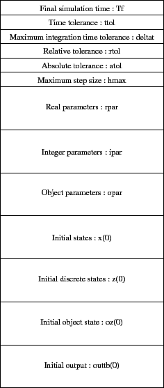
The map can also be accessible via a Xml file which is generated in the directory and is called Rdnom_params.xml. For i.e, the content of this file for the Scicos demo RLC_circuit.cosf is

<?xml version="1.0" encoding="ISO-8859-1"?>

<ScicosParam Name="RLC_circuit" version="scicos4.4">
  <ScicosVar name="tf" dim1="1" dim2="1" typ="10"/>
  <ScicosVar name="ttol" dim1="1" dim2="1" typ="10"/>
  <ScicosVar name="deltat" dim1="1" dim2="1" typ="10"/>
  <ScicosVar name="rtol" dim1="1" dim2="1" typ="10"/>
  <ScicosVar name="atol" dim1="1" dim2="1" typ="10"/>
  <ScicosVar name="hmax" dim1="1" dim2="1" typ="10"/>
  <ScicosVar name="rpar_1" dim1="1" dim2="1" typ="10"/>
  <ScicosVar name="rpar_2" dim1="7" dim2="1" typ="10"/>
  <ScicosVar name="rpar_3" dim1="6" dim2="1" typ="10"/>
  <ScicosVar name="ipar_2" dim1="12" dim2="1" typ="84"/>
  <ScicosVar name="ipar_3" dim1="10" dim2="1" typ="84"/>
  <ScicosVar name="x" dim1="3" dim2="1" typ="10"/>
  <ScicosVar name="outtb_1" dim1="1" dim2="1" typ="10"/>
  <ScicosVar name="outtb_2" dim1="1" dim2="1" typ="10"/>
</ScicosParam>

For each variable, the size and the type is given. One then can use an Xml parser, to read and write data in the parameters file.

Use of the functions getscicosparam and setscicosparam

The ScicosLab functions getscicosparam and setscicosparam can be used from the ScicosLab prompt to read and write data in the parameters file provided by the Scicos generation. It use the Xml file to know how is it written. For i.e, for the Scicos demo RLC_circuit.cosf :

Step 1 - Do the code generation.

    -->load SCI/macros/scicos/lib;
    -->exec(SCI+'/demos/scicos/Electrical/RLC_circuit.cosf',-1);
    -->[ok,scs_m,%cpr] = scicos_codegeneration(scs_m,list(1));
   

Step 2 - Run the standalone generated code with default values.

    -->[out1,out2]=RLC_circuit();
    -->scf(1);plot(out1.time,out1.values);

Step 3 - Load the parameters enclosed in the paramaters file in a ScicosLab list.

    -->curdir=getcwd();
    -->[dt,data] = getscicosparam(curdir+'/RLC_circuit/RLC_circuit_params.dat');

Step 4 - Change parameter values.

    -->dt(1)
    ans  =
             column 1 to 9

    !SicosParam  tf  ttol  deltat  rtol  atol  hmax  rpar_1  rpar_2  !

             column 10 to 15

    !rpar_3  ipar_2  ipar_3  x  outtb_1  outtb_2  !

    -->dt.tf=1;

Step 5 - Save the parameters list in the parameters file.

    -->ok=setscicosparam(dt,curdir+'/RLC_circuit/RLC_circuit_params.dat');

Step 6 - Re-Run the standalone generated code with new parameters values.

    -->[out1,out2]=RLC_circuit();
    -->scf(2);plot(out1.time,out1.values);

Authors

Scicos Team